Section 12 Example: Preprocessing workflow

In this example I walk through a preliminary exploration of one morphological variable in Komi-Zyrian dialects. I use general dplyr and purrr functions described in section Tools: R.

In principle there are four patterns that occur regularly: мунісныс, мунісны, муніны, муніныс. Only two first occur in this data, but the regex would in principle capture all of them.

The idea is to define a general function that with the simplest possible example data finds and classifies the wanted examples. This way we can differentiate the query and processing from the data we apply it into. So in principle we could take another Komi dialect sample and run similar analysis into that.

dummy_data <- tibble(token = c('мунісныс', 'мунісны', 'муніны', 'муніныс'))

filter_verbs <- function(data){
  data %>% mutate(type = if_else(str_detect(token, 'сн..$') & str_detect(token, 'с$'), 
                        true = 'isnɨs', 
                        false = if_else(str_detect(token, 'сн.') & str_detect(token, 'ы$'),
                                        true = 'isnɨ', 
                                        false = if_else(str_detect(token, '([^с]ныс$)'),
                                                                   true = 'inɨs', 
                                                                   false = 'inɨ')))) %>%
    mutate(type_final = as.factor(if_else(str_detect(type, 's$'), 
                                        true = 's-final', 
                                        false = 'vowel-final'))) %>%
    mutate(type_medial = as.factor(if_else(str_detect(type, 'sn'), 
                                        true = 's-medial', 
                                        false = 'vowel-medial')))
}

dummy_data %>% filter_verbs() %>% knitr::kable()

token	type	type_final	type_medial
мунісныс	isnɨs	s-final	s-medial
мунісны	isnɨ	vowel-final	s-medial
муніны	inɨ	vowel-final	vowel-medial
муніныс	inɨs	s-final	vowel-medial

It seems that the result is correct, so we can start to apply it to the real data. However, if we find problems along the way, we can always return to this point and modify the function, as long as we haven’t started to do manual edits in the derived files.

In the next step we load the corpus directly into R from previously saved RDS file. How these can be worked with was described in section Tools: R.

kpv <- read_rds('corpus.rds')

Of course if the corpus is small enough we can also just read it directly from whatever source we have. However, as this process is repeated every time we compile this website, it is easier to read it this way.

verbs <- kpv %>% 
  filter(! participant %in% c('NTP-M-1986', 'MR-M-1974', 'RB-1974')) %>% # this simply removes the western researchers Niko Partanen, Michael Rießler and Rogier Blokland
  filter(str_detect(token, '(и|і)(с)?ны(с)?$')) %>% # This selects the wanted tokens
  filter_verbs() %>% # Here we call the function we set up above
  select(token, type, everything())

We can easily look into how many types we have and which are the most common tokens. This doesn’t modify the data frame, but gives us information about how sensical the result is. Usually this kind of more finished document doesn’t show the whole workflow how the preprocessing function was edited iteratively while examination of the results shows something is off, but in principle older versions should usually be present in older Git commits. This can be useful when it is realized later that some of the older version was indeed the correct one.

verbs %>% count(type) %>% slice(1:10) %>% knitr::kable()

type	n
inɨ	300
inɨs	250
isnɨ	1803
isnɨs	1196

verbs %>% count(token) %>% arrange(desc(n)) %>% slice(1:10) %>% knitr::kable()

token	n
вӧліны	176
вӧліныс	113
кучисныс	84
воисныс	67
олісны	67
шуисны	57
локтісны	46
ветлісны	45
карисны	44
олісныс	44

verbs %>% filter(type == 'inɨs') %>% slice(1:10) %>% knitr::kable()

token	type	utterance	reference	participant	time_start	time_end	session_name	filename	word	type_final	type_medial
муніныс	inɨs	Нужник бӧкас сулалэ и бӧр муніныс.	kpv_izva19300000ArtijevI-135-10	IXA-M-18XX	90000	100000	kpv_izva19300000ArtijevI-135	/Volumes/langdoc/langs/kpv/kpv_izva19300000ArtijevI-135/kpv_izva19300000ArtijevI-135.eaf	муніныс	s-final	vowel-medial
муніныс	inɨs	Муніныс ныа вӧлӧн.	kpv_izva19570000-290_3bz-11	XXV-M-19XX	52900	54220	kpv_izva19570000-290_3bz-Bakur	/Volumes/langdoc/langs/kpv/kpv_izva19570000-290_3bz-Bakur/kpv_izva19570000-290_3bz-Bakur.eaf	Муніныс	s-final	vowel-medial
вӧліныс	inɨs	Баракъясас вӧліныс гразнӧйӧсь зэй.	kpv_izva19570000-290_3bz-23	XXV-M-19XX	111380	114420	kpv_izva19570000-290_3bz-Bakur	/Volumes/langdoc/langs/kpv/kpv_izva19570000-290_3bz-Bakur/kpv_izva19570000-290_3bz-Bakur.eaf	вӧліныс	s-final	vowel-medial
лэччаніныс	inɨs	Рытнас шонді лэччаніныс ке сӧстэм - мӧдасылас лоэ шондіа лун ,	kpv_izva19590000IgusevJA-280	JAI-M-1939	1104086	1109573	kpv_izva19590000IgusevJA	/Volumes/langdoc/langs/kpv/kpv_izva19590000IgusevJA/kpv_izva19590000IgusevJA.eaf	лэччаніныс	s-final	vowel-medial
лэччаніныс	inɨs	Шонді лэччаніныс ке гӧрд , мӧдасылас лоас тӧла лун .	kpv_izva19590000IgusevJA-288	JAI-M-1939	1165648	1169283	kpv_izva19590000IgusevJA	/Volumes/langdoc/langs/kpv/kpv_izva19590000IgusevJA/kpv_izva19590000IgusevJA.eaf	лэччаніныс	s-final	vowel-medial
уудиныс	inɨs	уудиныс (водьпомыс) ляпкыд.	kpv_izva19591216-05582_2az.29	MXV-F-1937	147886	150661	kpv_izva19591216-05582_2az	/Volumes/langdoc/langs/kpv/kpv_izva19591216-05582_2az/kpv_izva19591216-05582_2az.eaf	уудиныс	s-final	vowel-medial
лоиныс	inɨs	а сыри- сыритяяс ӧні нин лоиныс важынкаяс:	kpv_izva19591216-05582_4a.078	MXV-F-1937	519866	526876	kpv_izva19591216-05582_4a	/Volumes/langdoc/langs/kpv/kpv_izva19591216-05582_4a/kpv_izva19591216-05582_4a.eaf	лоиныс	s-final	vowel-medial
кӧйиныс	inɨs	кӧйиныс сёяс и кулэ.	kpv_izva19591216-05582_4a.101	MXV-F-1937	717843	720943	kpv_izva19591216-05582_4a	/Volumes/langdoc/langs/kpv/kpv_izva19591216-05582_4a/kpv_izva19591216-05582_4a.eaf	кӧйиныс	s-final	vowel-medial
кӧйиныс	inɨs	кӧйиныс верме кӧрлы джагедны и луна.	kpv_izva19591216-05582_4a.112	MXV-F-1937	774030	779556	kpv_izva19591216-05582_4a	/Volumes/langdoc/langs/kpv/kpv_izva19591216-05582_4a/kpv_izva19591216-05582_4a.eaf	кӧйиныс	s-final	vowel-medial
кӧйиныс	inɨs	кӧйиныс дебсе росся костэ;	kpv_izva19591216-05582_4a.113	MXV-F-1937	779556	783611	kpv_izva19591216-05582_4a	/Volumes/langdoc/langs/kpv/kpv_izva19591216-05582_4a/kpv_izva19591216-05582_4a.eaf	кӧйиныс	s-final	vowel-medial

Often the actual benefit of having the data in a programmatic environment instead of just ELAN is that can use in the research variables from metadata that cannot be accessed in ELAN. In our participant naming system we use usually the convention where the gender and birthyear are marked to the name id.

verbs <- verbs %>% mutate(gender = str_extract(participant, '(?<=-)[MF](?=-)')) %>%
  select(token, type, gender, participant, everything()) 

verbs %>%
  count(gender)

## # A tibble: 3 x 2
##   gender     n
##    <chr> <int>
## 1      F  2455
## 2      M  1029
## 3   <NA>    65

Here we see that for some speakers we didn’t find the gender specified as is described in the convention. The reason is that there are some old transcribed texts for which we don’t know who is the speaker – very likely the same text has been elicitated from several speakers and is some kind of a synthesis of those. We simply don’t know. This is somewhat typical for fieldwork data from the 19th and early 20th century, although variation in practices is also great. In this case we know (after looking a bit better which files are having this problem) what is the reason for this problem, and we can decide to leave out those cases if necessary. However, it is good to take into account that if there are missing values, it is very important to examine what is going on behind them.

verbs %>%
  filter(is.na(gender)) %>%
  count(type)

## # A tibble: 4 x 2
##    type     n
##   <chr> <int>
## 1   inɨ     7
## 2  inɨs     3
## 3  isnɨ    52
## 4 isnɨs     3

In this point we can take a note that in the oldest data available there are very few examples of the s-final forms, but it is also a very small subset of the corpus.

Before advancing further, we can add one more variable to the dataframe we are working with.

verbs <- verbs %>% 
  mutate(year = str_extract(session_name, '\\d{4}(?=\\d{4})')) %>% 
  select(token, type, gender, year, everything())

Year is of course a bit problematic variable as we aren’t really having that much data for each year. So let’s add a new column for the decade.

verbs <- verbs %>% 
  mutate(type = as.factor(type)) %>%
  mutate(year = as.numeric(year)) %>%
  mutate(decade = (year %/% 10) * 10) %>%
  select(token, type, gender, year, decade, everything())

After this the plotting will work nicely. We can analyze the distribution of tokens per decade:

ggplot(verbs,
       aes(x = decade)) +
  geom_bar()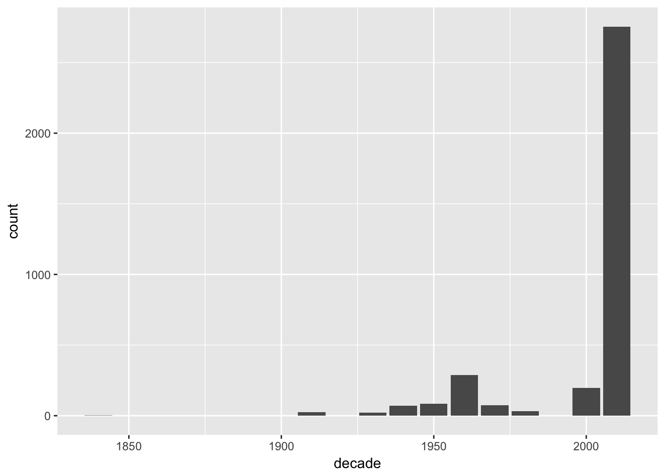

This reflects well the data distribution of IKDP corpus, which makes sense as these verb forms should occur everywhere.

ggplot(verbs) + 
  geom_bar(mapping = aes(x = decade, fill = type_medial), position = "fill")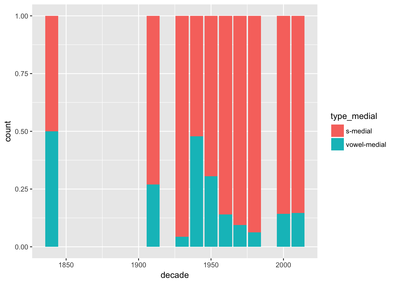

ggplot(verbs %>%
         filter(year > 1930)) + # This leaves older data out as it is so gappy
  geom_bar(mapping = aes(x = decade, fill = type_medial), position = "fill")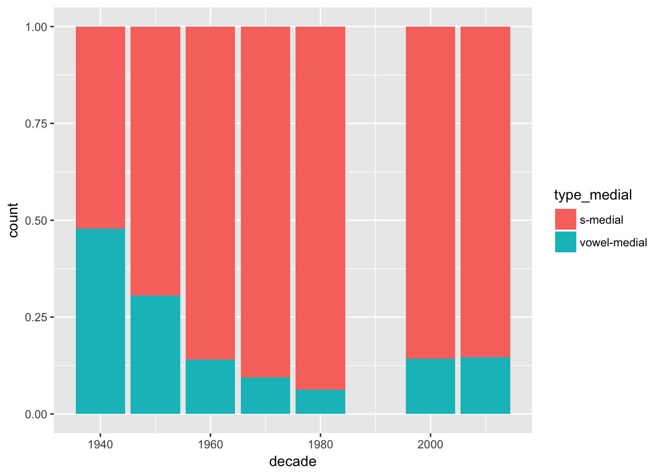

ggplot(verbs %>%
         filter(year > 1930) %>%
         filter(! is.na(gender))) + # If we want to use a variable later, we have to make sure it is available
  geom_bar(mapping = aes(x = decade, fill = type_medial), position = "fill") +
  facet_grid(. ~ gender)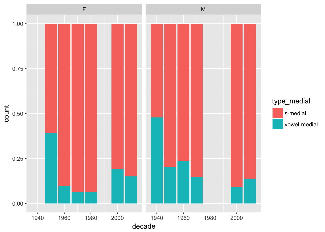

Next thing I want to try is to associate birth places with areas and plot those. For this we need bit more metadata, which I’m now reading from our Filemaker Pro database, but which should be set up better for the actual teaching.

Once we have set up the processing workflow to the point where we have something useful, and maybe get into phase where we don’t know what we are doing, it can be an useful practice to write the dataframe into a new variable so that it is not necessary to do all previous changes when something goes wrong. In this case I create a new variable called verbs_test, and when we accidentally do something we didn’t want to it is easy to run the code from this point onward.

source('/Volumes/langdoc/langs/kpv/FM_meta.R')

## Loading required package: DBI

## Loading required package: rJava

## Joining, by = "Actor_ID"

## Joining, by = "Session_ID"

## Joining, by = "RecPlace_OSM_ID"

## Joining, by = "PlaceofRes_OSM_ID"

## Joining, by = "Birthplace_OSM_ID"

## Warning in eval(ei, envir): NAs introduced by coercion

## Warning in eval(ei, envir): NAs introduced by coercion

## Warning in eval(ei, envir): NAs introduced by coercion

## Warning in eval(ei, envir): NAs introduced by coercion

## Warning in eval(ei, envir): NAs introduced by coercion

## Warning in eval(ei, envir): NAs introduced by coercion

## Warning in eval(ei, envir): NAs introduced by coercion

# meta %>% distinct(place_birth, birthplace_osm_id, lat_birth, lon_birth) %>% 
#   arrange(place_birth) %>% 
#   group_by(place_birth) %>% 
#   filter(n()>1)

verbs_test <- left_join(verbs, meta %>% distinct(participant, lat_birth, lon_birth, attr_foreign) %>% filter(participant %in% verbs$participant)) %>%
  rename(lat = lat_birth,
         lon = lon_birth)

## Joining, by = "participant"

verbs_test <- verbs_test %>% 
  mutate(variety = str_extract(session_name, '(?<=kpv_)[a-z]+'))

12.1 From points to polygon

#izva <- st_read('https://raw.githubusercontent.com/langdoc/IKDP-2/025e817c25181b683661a21ab36facb63c830604/data/izva_dialects.geojson')

izva <- st_read('/Users/niko/github/IKDP-2/data/izva_dialects-test.geojson')

## Reading layer `OGRGeoJSON' from data source `/Users/niko/github/IKDP-2/data/izva_dialects-test.geojson' using driver `GeoJSON'
## Simple feature collection with 19 features and 4 fields
## geometry type:  POLYGON
## dimension:      XY
## bbox:           xmin: 28.96325 ymin: 55.94814 xmax: 74.33177 ymax: 70.39286
## epsg (SRID):    4326
## proj4string:    +proj=longlat +datum=WGS84 +no_defs

ggplot(izva) +
  geom_sf(aes(fill = variant)) +
  geom_point(data = verbs_test %>% filter(! is.na(lon)),
             aes(x = lon, y = lat))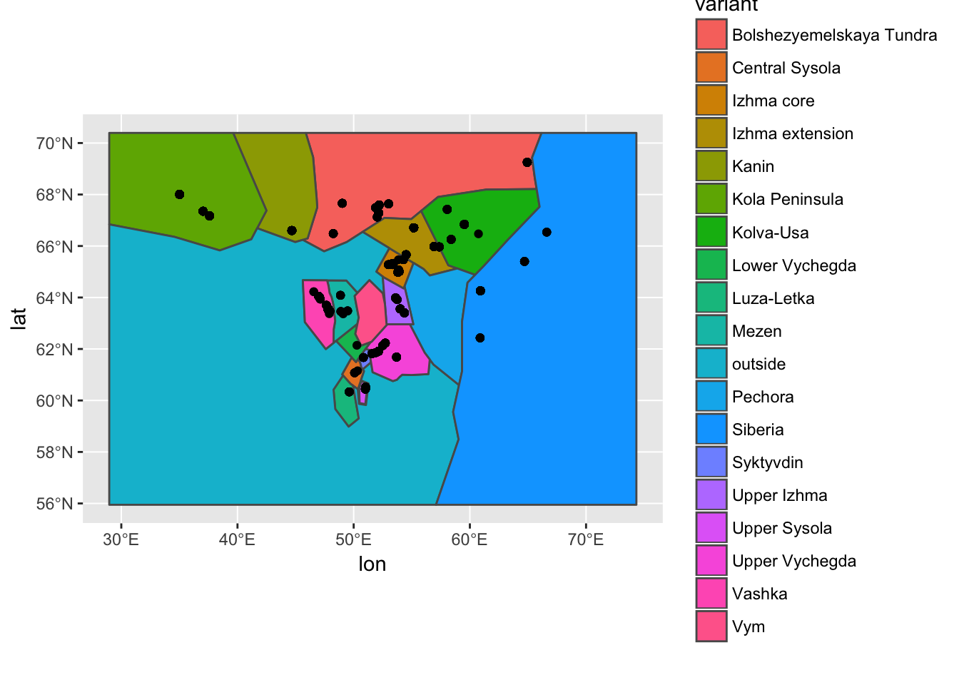

verbs_test %>% filter(is.na(lat)) %>% count(participant) %>% arrange(desc(n))

## # A tibble: 31 x 2
##    participant     n
##          <chr> <int>
##  1  IIB-M-1946    58
##  2  TFA-F-1934    46
##  3  APP-F-1957    39
##  4     unknown    25
##  5  AAZ-F-1940    20
##  6  KOM-F-1964    13
##  7  XXC-F-196X     8
##  8  NGK-F-1956     6
##  9      группа     6
## 10          S1     5
## # ... with 21 more rows

## based on this:
## https://gis.stackexchange.com/questions/222978/lon-lat-to-simple-features-sfg-and-sfc-in-r

geo_inside <- function(lon, lat, map, variable) {

  variable <- enquo(variable)
  pt <-
    tibble::data_frame(x = lon,
                       y = lat) %>%
    st_as_sf(coords = c("x", "y"), crs = st_crs(map))
  pt %>% st_join(map) %>% pull(!!variable)

}

verbs_test <- verbs_test %>% 
  filter(! is.na(lon) | ! is.na(lat)) 

verbs_test %>% count()

## # A tibble: 1 x 1
##       n
##   <int>
## 1  3281

verbs_test <- verbs_test %>% 
  mutate(region = geo_inside(lon, lat, izva, variant))

## although coordinates are longitude/latitude, it is assumed that they are planar

verbs_test <- verbs_test %>% 
  mutate(dialect = geo_inside(lon, lat, izva, dialect))

## although coordinates are longitude/latitude, it is assumed that they are planar

ggplot(data = verbs_test %>%
         filter(str_detect(dialect, 'zva')),
       aes(x = type)) +
  geom_bar() +
  facet_wrap(region ~ gender)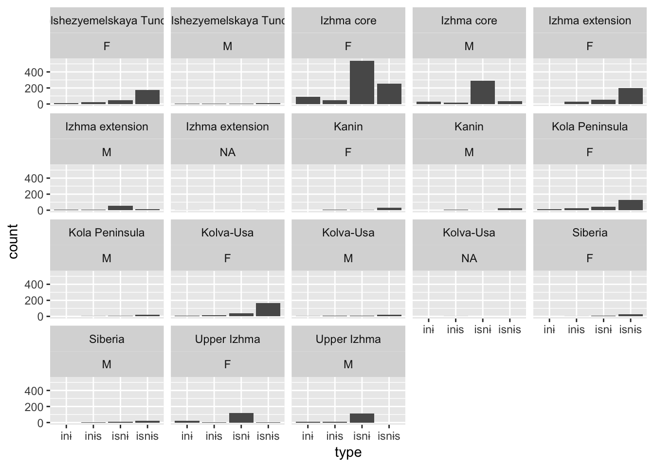

verbs_test %>% count(dialect)

## # A tibble: 9 x 2
##          dialect     n
##           <fctr> <int>
## 1 Central Sysola     6
## 2           izva  1311
## 3           Izva  1566
## 4 Lower Vychegda     1
## 5     Luza-Letka    12
## 6      Syktyvdin     7
## 7          Udora   257
## 8   Upper Sysola    30
## 9 Upper Vychegda    91

ggplot(verbs_test %>%
         filter(! is.na(region)) %>%
         filter(str_detect(dialect, 'zva'))) +
  geom_bar(mapping = aes(x = region, fill = type), position = "fill") +
theme(axis.text.x = element_text(angle = 90, hjust = 1))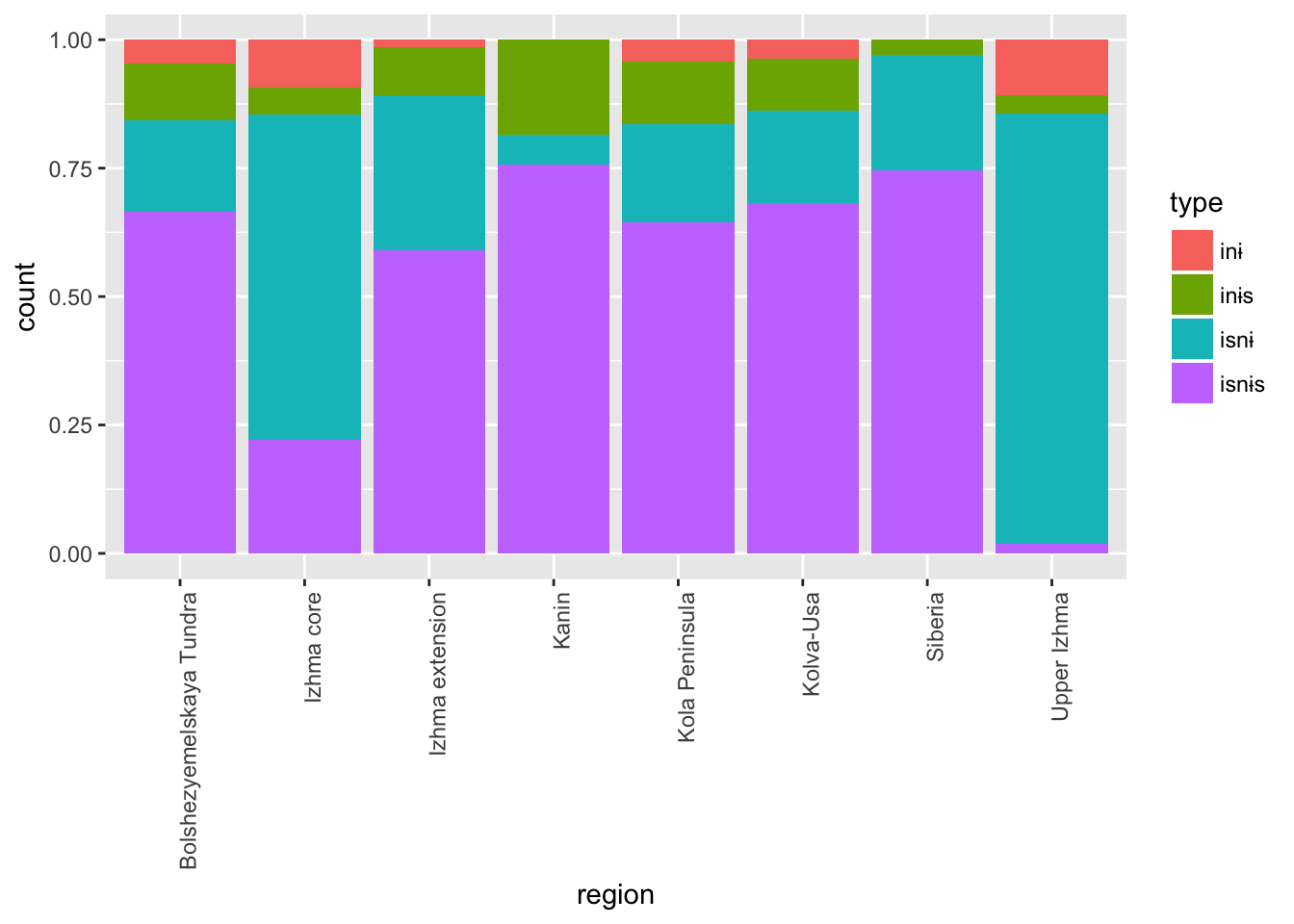

ggplot(verbs_test %>%
         filter(! participant %in% c('MSF-F-1968', 'VPC-M-1993')) %>%
         filter(! is.na(region)) %>%
         filter(str_detect(dialect, 'zva'))) +
  geom_bar(mapping = aes(x = region, fill = type), position = "fill") +
theme(axis.text.x = element_text(angle = 90, hjust = 1))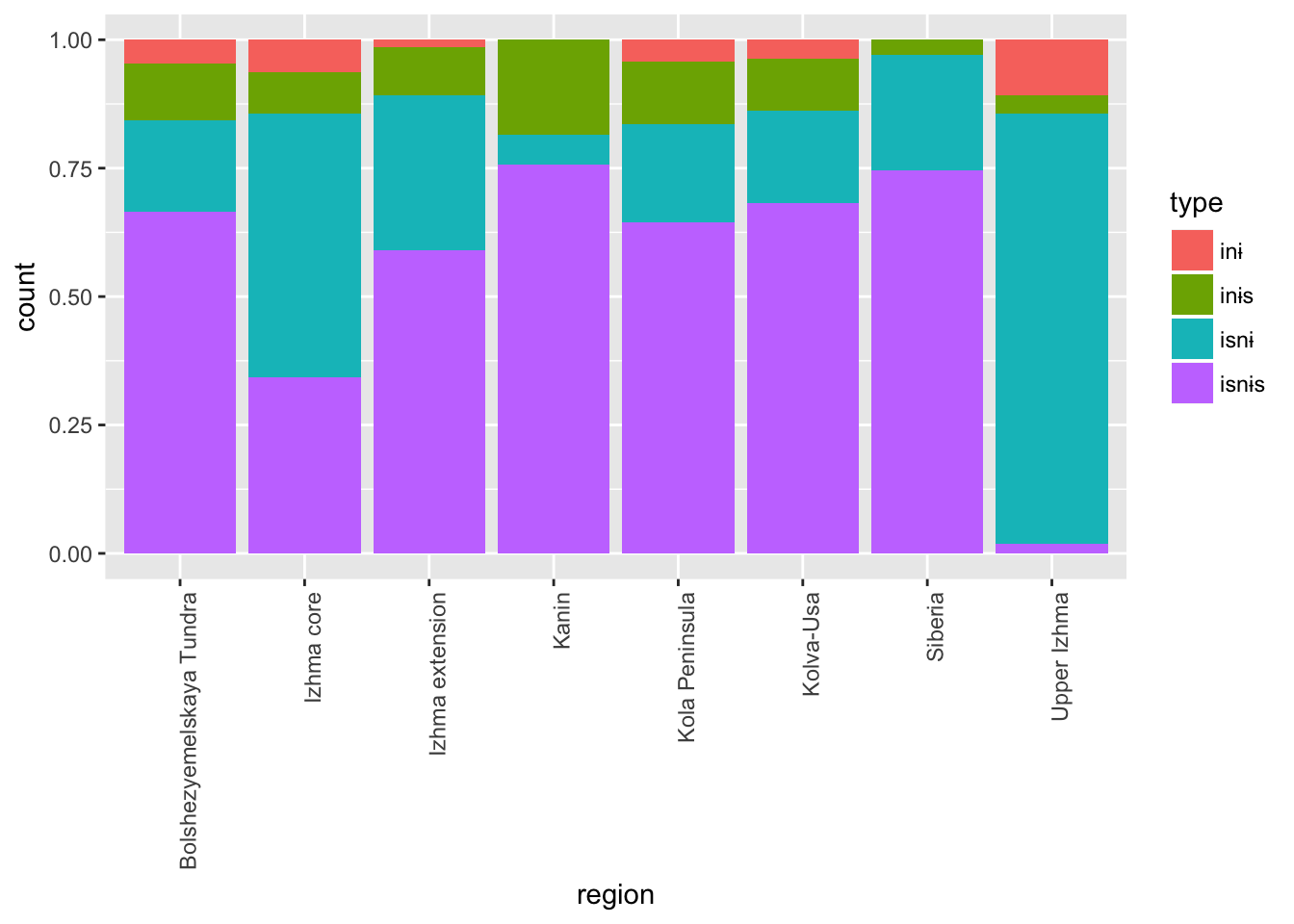

library(geofacet)

mygrid <- data.frame(
  code = c("IZKA", "IZKP", "IZBT", "IZCO", "IZSIB", "IZEX", "IZKU", "UDVA", "UDMZ", "VM", "IZUP", "PE", "VYLO", "VYUP", "SK", "SD", "SC", "LL", "SU"),
  name = c("Kanin", "Kola Peninsula", "Tundra", "Izhma core", "Siberia", "Izhma extension", "Kolva-Usa", "Vashka", "Mezen", "Vym", "Upper Izhma", "Pechora", "Lower Vychegda", "Upper Vychegda", "Syktyvkar", "Syktyvdin", "Central Sysola", "Luza-Letka", "Upper Sysola"),
  row = c(1, 1, 1, 2, 2, 2, 2, 3, 3, 3, 3, 3, 4, 4, 5, 6, 7, 7, 8),
  col = c(2, 1, 3, 4, 7, 5, 6, 1, 2, 3, 4, 5, 3, 4, 3, 3, 4, 2, 5),
  stringsAsFactors = FALSE
)
geofacet::grid_preview(mygrid)

## You provided a user-specified grid. If this is a generally-useful
##   grid, please consider submitting it to become a part of the
##   geofacet package. You can do this easily by calling:
##   grid_submit(__grid_df_name__)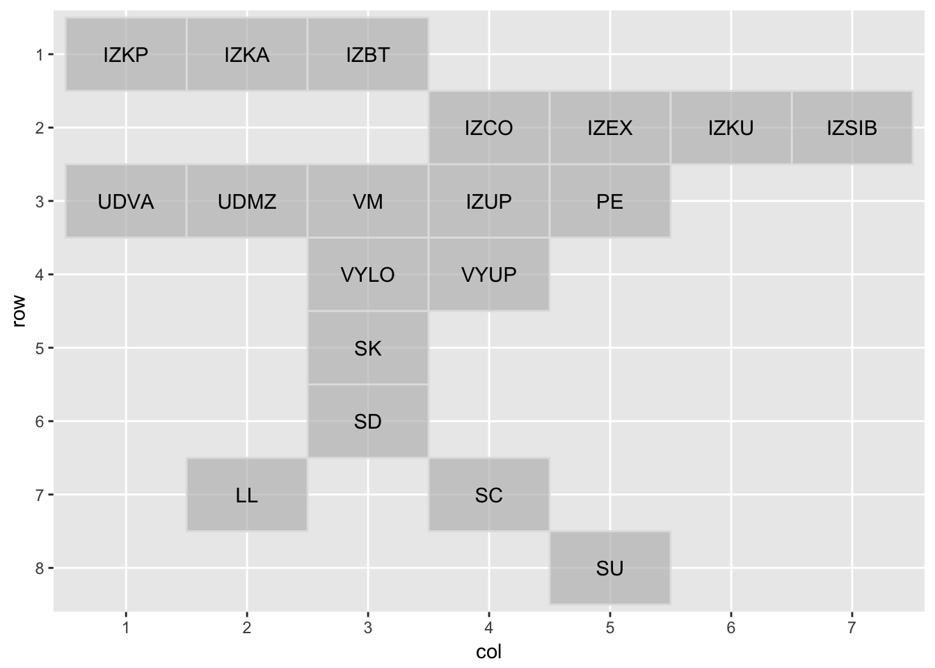

# verbs_test %>% mutate(name = as.character(region)) %>%
#          mutate(name = if_else(name == 'Bolshezyemelskaya Tundra', 'Tundra', name)) %>%
#          left_join(mygrid) %>%
#          filter(! is.na(region)) %>% filter(variety == 'vym') %>% select(name)

ggplot(verbs_test %>% 
         mutate(name = as.character(region)) %>%
         mutate(name = if_else(name == 'Bolshezyemelskaya Tundra', 'Tundra', name)) %>%
         left_join(mygrid) %>%
         filter(! is.na(region)) %>%
         filter(! participant %in% c('MSF-F-1968', 'VPC-M-1993', 'VVF-F-1957'))) +
  geom_bar(mapping = aes(x = factor(""), fill = type), position = "fill") +
  facet_geo(~ name, grid = mygrid) + 
  labs(title = "First preterite plural verb allomorphs in Komi-Zyrian dialects",
       subtitle = "Map approximates the location and contact relations of the dialects. For blanks no data available.",
    caption = "Work done in LATTICE, Paris\nData Source: IKDP Author: Niko Partanen (2017)",
    y = "Percentage of different types",
    x = "") +
  theme_bw() +
  theme(axis.line=element_blank(),
      axis.text.x=element_blank(),
      axis.text.y=element_blank(),
      axis.ticks=element_blank(),
#      axis.title.x=element_blank(),
#      axis.title.y=element_blank(),
#      legend.position="none",
      panel.background=element_blank(),
#      panel.border=element_blank(),
      panel.grid.major=element_blank(),
      panel.grid.minor=element_blank()) +
  theme(strip.background = element_rect(fill="white", linetype = 'blank'))+
  theme(strip.text = element_text(colour = 'black', size = 7))

## Joining, by = "name"

## You provided a user-specified grid. If this is a generally-useful
##   grid, please consider submitting it to become a part of the
##   geofacet package. You can do this easily by calling:
##   grid_submit(__grid_df_name__)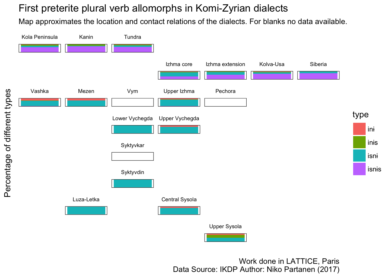

# ggplot(verbs_test %>%
#          filter(! participant %in% c('MSF-F-1968', 'VPC-M-1993')) %>%
#          filter(! is.na(region)) %>%
#          filter(! is.na(gender)) %>%
#          filter(str_detect(dialect, 'zva'))) +
#   geom_bar(mapping = aes(x = gender, fill = type), position = "fill") +
# theme(axis.text.x = element_text(angle = 90, hjust = 1))
# 


ggplot(verbs_test %>%
         filter(! is.na(region)) %>%
         filter(! str_detect(dialect, 'zva'))) +
  geom_bar(mapping = aes(x = region, fill = type), position = "fill") +
theme(axis.text.x = element_text(angle = 90, hjust = 1))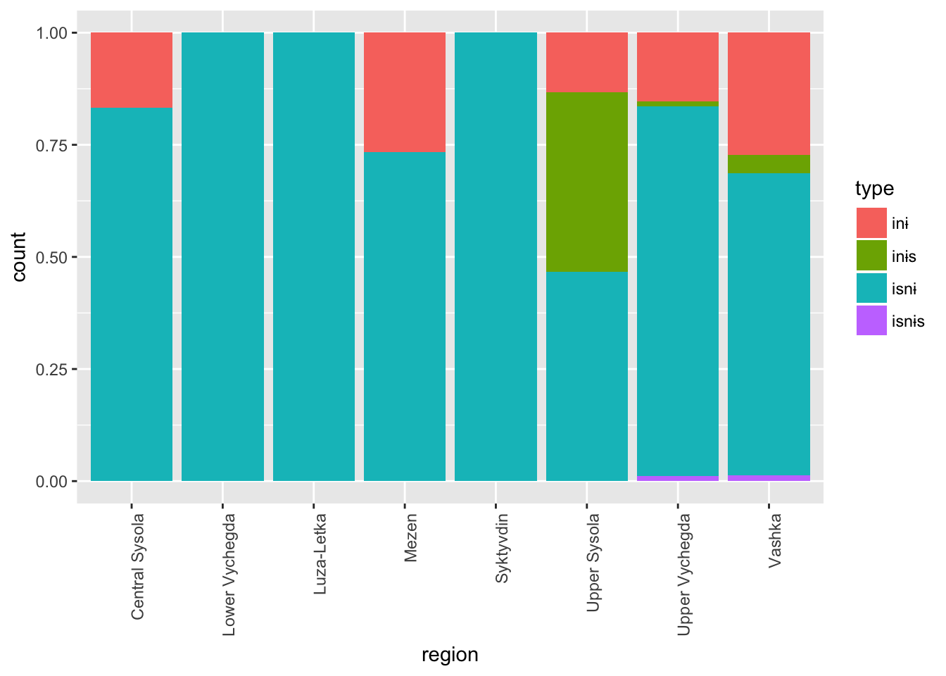

# verbs_test %>% filter(type == 'inɨ')

verb_stems <- verbs_test %>% 
  mutate(stem = str_extract(token, '.+(?=(и|і)с?ны?с?)')) %>% 
  distinct(stem) %>% 
  arrange(stem)

# verb_stems %>% 
#   filter(! str_detect(stem, "(j|['])")) %>%
#   write_csv('data/izva_verbs.csv')

# verbs_test %>% 
#   mutate(stem = str_extract(token, '.+(?=(и|і)с?ны?с?)')) %>% 
#   count(stem) %>%
#   arrange(desc(n)) %>%
#   slice(10:20)

# verbs_test %>% 
#   filter(variety == 'izva') %>%
#   mutate(stem = str_extract(token, '.+(?=(и|і)с?ны?с?)')) %>%
#   filter(! stem == 'в') %>%
#   count(stem, type) %>%
#   rename(hits = n) %>%
#   arrange(stem) %>%
#   split(.$stem) %>%
#   map(~ mutate(.x, diff_types = n()) %>%
#         mutate(type_ratio = hits / sum(hits)) %>%
#         mutate(sum_hits = sum(hits))) %>%
#   bind_rows %>%
#   filter(sum_hits > 10) %>%
#   arrange(desc(diff_types)) %>% View
  
# verbs_test %>% 
#   filter(variety == 'izva') %>%
#   mutate(stem = str_extract(token, '.+(?=(и|і)с?ны?с?)')) %>%
#   filter(stem == 'босьт') %>%
#   filter(type == 'isnɨs') %>%
#   select(utterance) %>%
#   View

# verbs_test %>% filter(str_detect(utterance, 'всю')) %>% select(utterance, filename) %>% open_eaf(3)
# kpv  %>% filter(str_detect(utterance, 'кеде ')) %>% distinct(utterance, participant, filename) 
# 
#   split(.$type) %>%
#   map(~ count(.x, stem) %>%
#           arrange(desc(n)) %>%
#           slice(10:20))


# verbs_test %>% filter(str_detect(token, '^кор')) %>% select(utterance, participant, variety, year)
# verbs_test %>% filter(str_detect(token, '^торйед')) %>% open_eaf(1)

verbs_test %>% 
  mutate(stem = str_extract(token, '.+(?=(и|і)с?ны?с?)')) %>% 
  left_join(read_csv('data/izva_verbs.csv')) %>% 
  filter(! is.na(category)) %>% 
  filter(stem != 'вӧл') %>%
#  select(token, type, type_medial, gender, year, participant, category, variety, region, dialect) %>%
  ggplot(data = .,
         aes(x = category)) +
  geom_bar() +
  facet_grid(. ~ type)

## Parsed with column specification:
## cols(
##   stem = col_character(),
##   category = col_character(),
##   remove = col_character()
## )

## Joining, by = "stem"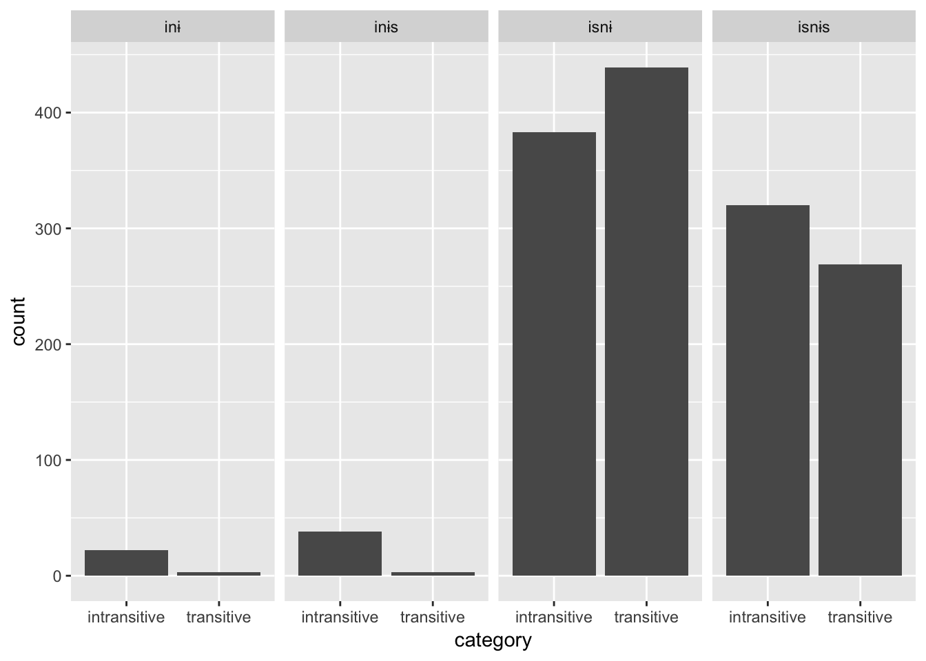

verbs_test %>% 
  mutate(stem = str_extract(token, '.+(?=(и|і)с?ны?с?)')) %>% 
  left_join(read_csv('data/izva_verbs.csv')) %>% 
  filter(! is.na(category)) %>% 
  filter(dialect %in% c('Udora', 'izva', 'Izva')) %>%
  filter(stem != 'вӧл') %>%
  select(token, type, gender, year, participant, category, variety, region, dialect) %>%
  ggplot(data = .,
         aes(x = category)) +
  geom_bar() +
  facet_grid(type ~ variety)

## Parsed with column specification:
## cols(
##   stem = col_character(),
##   category = col_character(),
##   remove = col_character()
## )
## Joining, by = "stem"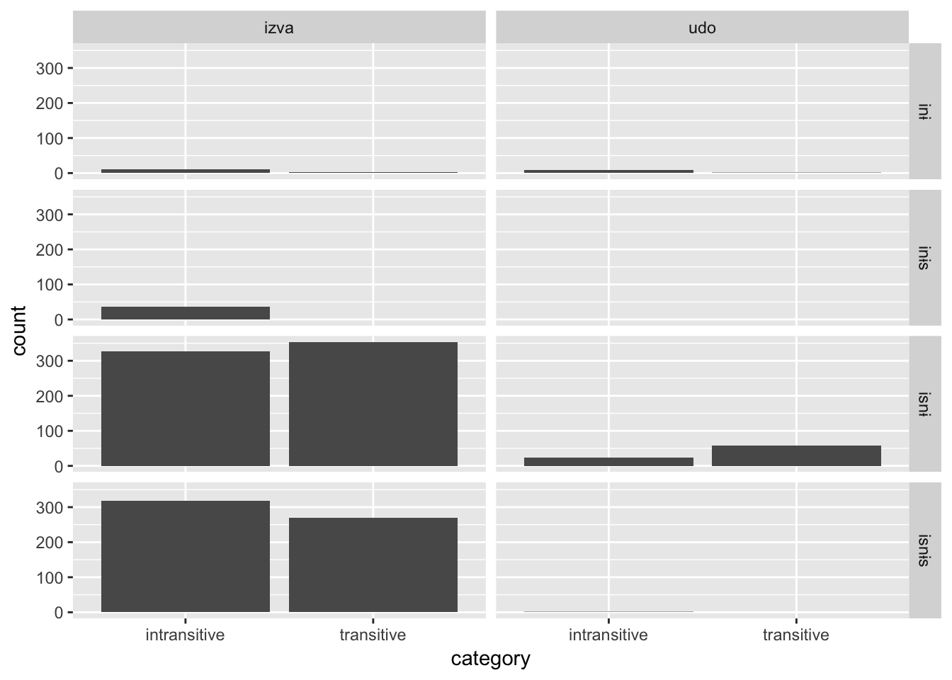

int <- verbs_test %>% 
  mutate(stem = str_extract(token, '.+(?=(и|і)с?ны?с?)')) %>% 
  left_join(read_csv('data/izva_verbs.csv')) %>% 
  filter(! is.na(category))

## Parsed with column specification:
## cols(
##   stem = col_character(),
##   category = col_character(),
##   remove = col_character()
## )
## Joining, by = "stem"

# int %>% 
#   left_join(count(int, stem) %>% rename(token_count = n)) %>% 
#   arrange(desc(token_count)) %>%
#   distinct(stem, token_count) %>%
#   ggplot(data = .,
#          aes(x = token, y = token_count)) +
#   geom_bar()

# блиныс

# verbs %>% arrange(token) %>% distinct(token) %>% write_csv('data/izva_verbs.csv')

# verbs %>% filter(str_detect(token, 'j'))

# verbs %>% mutate(variant = str_extract(session_name, '(?<=kpv_)[a-z]+(?=\\d)')) %>% count(variant)
#verbs %>% left_join()